A short introduction to krystals
Put simply, a krystal is an abstract data type which can store large amounts of hierarchically organised material. This is my contribution to the fields of serial technique and algorithmic composition.
It would have been difficult to have written my curriculum vitae without mentioning krystals, so this site would be incomplete without giving some idea of what they are. Understanding krystals is necessary for understanding my work as a whole (for example, why I started programming as early as 1982), but is not necessary for understanding the rest of this site (Stockhausen scores, FreeHand Xtras, The Notation of Time etc.). This is because symbols dont have to be contained in krystals, and because a krystal’s structure is independent of the symbols it contains.
My object here is simply to describe what a krystal is, and what this data type implies. I also have included some examples of krystals, expressed as formatted numbers. My (unpublished) KRYSTALS software 1 has extensive documentation, including a more complete description of the algorithms, file structures etc. If anyone is interested, they will doubtless let me know....
Krystals are perhaps best understood by following the steps I took while developing them. This development took place in two major phases - 1969-73 and 1978-93, so this document falls naturally into two parts.
Part 1: 1969-73 Expansions and Fields
Terms defined in this section are:
As a student at the Royal Academy of Music (1968-72), I took part in James
Iliff’s weekly seminars for composers. These were a good place for brainstorming...
At one of these seminars, one of the students brought along a copy of WATT
2 by Samuel Becket. This is a funny novel, containing a piece of ‘music’
for three frogs. Here is how it starts:
| Krak! | - | - | - | - | - | - | - | Krak! | - | - | - | - | - | - | - | Krak! | etc. |
| Krek! | - | - | - | - | Krek! | - | - | - | - | Krek! | - | - | - | - | Krek! | - | etc. |
| Krik! | - | - | Krik! | - | - | Krik! | - | - | Krik! | - | - | Krik! | - | - | Krik! | - | etc. |
The frogs continue to croak at their prescribed intervals (8, 5, 3) until they all croak at once (at the 121st time unit).
We performed this at the seminar, and for a few weeks were occupied with variations on this theme...
This lead me to a general idea for constructing large accumulations of material with a particular ‘colour’ by dividing a long line into different numbers of parts for the elements contained. For example, the line below has 67 green divisions, and 17 red divisions:
Definition: the above line has domain 2 (the number of different elements).
Such a line can have any domain, and any proportion between the amounts of each element.
I was very soon using this technique to generate pitches, ignoring the exact spacing on the line, but reading off the pitches from left to right.
The problem now arises as to where I find the proportions into which the line is to be divided. In particular, how do I invert a proportion to get from

There is a geometrical way of doing this. Consider a close-up of a section of the above two lines:
Joining successive green intersections, and successive red intersections gives:
It can be proven quite easily, that the green connectors all cross at a focus, and that it doesnt matter which pair of green points one joins first - the focus is always at the same height above the top black line. Simlarly for the red connectors. Those not inclined to do any elementary geometry might like to note that this construction bears a close resemblance to the one used in perspective drawing... A set of parallel green lines receding into the distance...
There is a practical problem here, in that it is difficult to construct all the connectors because they get very close together as they get more horizontal. I solved this problem, and the problem of organically changing hierarchies by using trammels.
Definition: a trammel is a piece of paper, along the edge of which ‘expansion distances’ are drawn. For example, the trammel for the top hierarchy in the above diagram contains only one green and one red distance:
Definiton: an expansion is created by setting the trammel’s origin to the most recent occurrence of each element in turn, and setting off its ‘expansion distance’ to find the position of the next occurrence. Changing trammels on an expansion is no problem, providing they share the same domain (number of different elements). The join, where trammels change, is completely ‘organic’: the local context at the point of growth is all that matters...
Notice that g/r is equal to G/R in the following diagram:
So, as far as trammels are concerned, I can use G and R instead of g and r. The diagram can be replaced simply by the two foci, and an organic expansion can be made as follows:
Definition: I call the line of results
from a single trammel a strand.
Note that I am only interested in the sequence of the elements - the spaces
between them are only a measure of the likelihood of their occurrence. The above expansion
defines the sequence:

This is all well and good for a domain of 2 elements, but I want to be able to have any domain. The problem is that the foci, and the points from which trammels are constructed, are all on one line (in one dimension). Only the vertical distance between a focus and a trammel-point matters. This means, in the following example, that I cant move from green to red without going near blue. It also means that there is nowhere, except an infinite distance away to the top or bottom of the diagram, where the elements all have equal distances on a trammel.
Consider what happens when the foci and trammel-points are allowed to be in two dimensions. Trammels are now constructed by measuring the shortest distance3 between the trammel-point and the foci in any direction on the page:
If there is to be an accessible trammel-point equidistant from all the foci, then the foci must lie on a circle with that point at the centre:
Note that:
I also use the terms ‘absolute hierarchy’ and ‘eccentricity’ in relation to strands, because a strand has a direct relation to a trammel.
I now want to describe the geographies of two major groups of fields, each having regularly spaced foci. Having regularly spaced foci ensures the foci are as independent as possible. If two foci are close together, then one cannot be approached without approaching the other.
The first group has its foci distributed around a semicircle.
Definition: I call fields having foci regularly
distributed on a semicircle linear fields.
Linear fields are useful for parameters having a natural linear order - for example dynamics
from pppp to ffff, or densities, or eccentricities. A linear field with domain 8 looks like:
The absolute hierarchies in this field are to be found in segments of the circle with borders passing through the foci and midway between the foci:
The absolute hierarchies in these segments are (with the most predominant element on the left of the hierarchy):
The form of this permutation of the elements in the absolute hierarchies is characteristic for linear fields. A similar permutation arises in any domain. To be absolutely clear: an absolute hierarchy is associated with a particular segment because all trammels constructed from points in that segment share the same absolute hierachy.
The second group of fields has its foci distributed around a complete circle.
Definition: I call fields having foci regularly
distributed around a complete circle circular fields.
Such fields are apropriate for all parameters which have a naturally circular order, or no
natural order at all - for example the absolute pitches a-flat, D-flat, E-natural etc.
Here is a circular field4 with domain 8:
The order in which the foci are labelled has no significance, except that I wanted the first hierarchy above focus 1 to be 12345678 (see below). Again, absolute hierarchies change at the borders of segments which pass through foci or the mid points between foci:
As with linear fields, this arrangement also gives rise to a characteristic permutation of the elements in the absolute hierarchies:
This is (literally) a multiple helix projected into the plane of the page.
When expanding a strand, three values are initially required:
density - the number of elements in the completed
strand
eccentricity - the degree of imbalance in the hierarchy
absolute hierarchy - the order of prevalence of
the elements
The completed strand may contain many elements. This implies that expansion is a way of getting
from one level of detail to another. Consider what happens if the three inputs are themselves
strands:
density (D): 556758
eccentricity (E): 453627
absolute hierarchy (H): 115342
Explaining the precise meanings of the eccentricity and absolute hierarchy inputs goes
beyond the scope of this document, but note that expanding with these three strands results
in 6 new strands:
| density | eccentricity | absolute hierarchy | new strand (e.g.) | |
| Strand 1 input: | 5 | 4 | 1 | 11432 |
| Strand 2 input: | 5 | 5 | 1 | 12341 |
| Strand 3 input: | 6 | 3 | 5 | 553454 |
| Strand 4 input: | 7 | 6 | 3 | 6354217 |
| Strand 5 input: | 5 | 2 | 4 | 44344 |
| Strand 6 input: | 8 | 7 | 2 | 63245712 |
I call this block of new strands a level 2 krystal. A level 1 krystal contains a single strand. a level 0 krystal contains a single value (a constant). A level 3 krystal can be produced by expanding level 2 krystals. There is no limit to the number of levels a krystal may have (the single notes in beyond the symbolic were at level 8). See also: examples of krystals
Note also that the krystal inputs to an expansion dont all have to have the same level - they simply need to share the same density structure at some level. For example, the three inputs above are all level 1 krystals with density 6. One or two of the inputs could, however, have been constant (e.g. E=6). My current expansion program (xk) therefore has an independent level input which defines the level of the output, in addition to the original density, eccentricity and hierarchy krystal inputs.
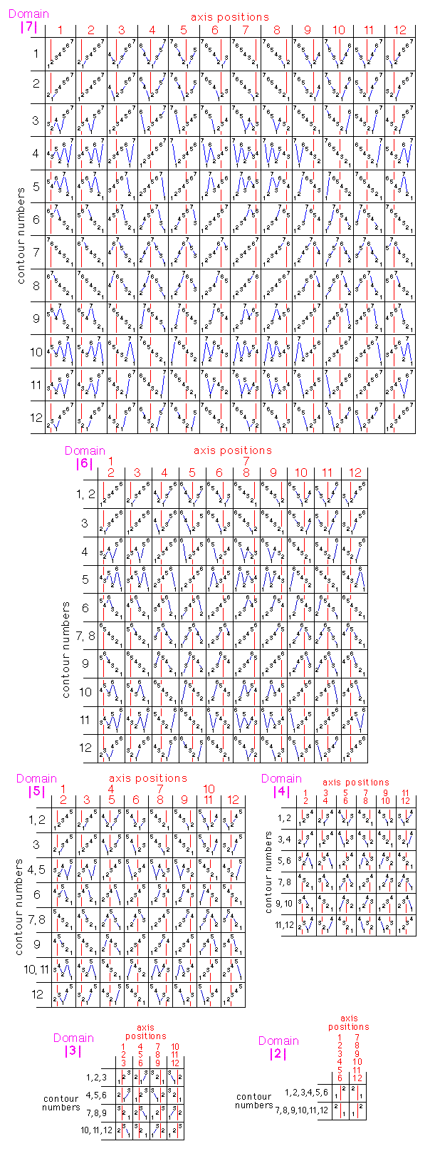
A further refinement of xk, is that it takes ‘axis’ and ‘contour’ krystal inputs. These define the internal permutation (shape) of each strand. I regard the order of the values within a strand, which results from the expansion, as being essentially outside time. A strand is, like a beamed group of notes, a word-like object whose internal structure needs to be related to the internal structure of other strands in order to carry meaning. This is, for me, the beginning of an attempt to reestablish a kind of counterpoint as a structural principle... (Not just the counterpoint of pitches 5 which is obvious in ‘beyond the symbolic’ , but a general counterpoint of all parameters at all levels of detail.)
The values in the axis and contour input krystals are the coordinates in tables of standard permutations. For these coordinates to make sense, neigbouring permutations in the tables must be related. In ‘beyond the symbolic’, I used the following ‘spherical’ 6 tables (spherical because both the axis and contour coordinates are circular functions). Note that these tables are ‘concentric’, in that contour numbers and axis positions are related across different domains. Note also that inverted permutations are to be found at diametrically opposed positions (‘contrary motion’).